1. Introduction

Wheat is the most traded staple food and it is grown on a larger area than any other crop. It has long been a staple in many countries and is widely consumed, even in places where its production is virtually impossible. Contrary to other staples, such as rice, it can be preserved and stored quite easily. This helps to explain its predominant role within the total agricultural trade. Wheat-based products have been at the core of many countries’ diets, so the functioning of the international wheat market has often been crucial for world food security. Agricultural policy –including commercial policy– has always paid special attention to wheat, both in industrialized and in developing countries. Wheat has been the most important traded food for low-income countries and the major component of food aid (Callear & Blandford, 1981). It also played a key role in geo-strategic relations during the Cold War period (Morgan, 1979) and has been a chief protagonist in major technological changes in agricultural methods and plant breeding (Perkins, 1997).

This paper aims to identify the main drivers of world wheat trade over the period 1963-2010. More specifically, it is concerned with the factors that explain the geographical distribution of the wheat trade (bilateral trade flows). For that purpose, we follow a cliometric approach. First, we consider the historical and institutional framework of the wheat trade over the studied period. This framework was deeply affected by the pre-war situation in wheat markets, and consolidated its distinctive and longstanding characteristics over the immediate post-war years. The history of the trade cannot be detached from the very peculiar institutional configuration that ruled the world agricultural trade after Second World War. This framework evolved over time, certainly affecting the volume and direction of wheat trade flows. Further complicating matters is the fact that national and international wheat policies implemented throughout this period were usually the result of economic policy goals that were not directly related to wheat. While in some countries wheat policies were primarily driven by the aim of assuring farmers a “fair” income, in other countries wheat policies were fundamentally aimed at achieving self-sufficiency in food. In other cases, wheat policies were designed to solve balance of payments problems. The trade in wheat does not occur in an empty geopolitical/institutional space, but in a very complex institutional framework that is resistant to analysis, let alone to incorporate in an econometric model. There are, however, powerful physical and economic forces that explain a substantial part of the observed wheat trade flows. This is why we estimate several econometric models based on the gravity principle of international trade and discuss the results, taking into account the historical/institutional conditions that prevailed in wheat markets over the studied period.

The paper is structured as follows. A rough description of the evolution of the world wheat trade between 1939 and 2010 is carried out in section 2. This section also draws on other academic and historical sources to depict the institutional and geopolitical background in which the trade occurred. Section 3 deals with the theoretical and empirical foundations of the gravity equation (GE), and discusses the advantages of using the Poisson pseudo maximum likelihood estimator (PPML) over other alternative estimation methods for our case study. The dataset is presented in Section 4, in which several econometric models are also estimated and discussed. The main conclusions of the paper are set out in Section 5.

2. The world wheat market

It is well known that wheat markets experienced serious troubles during the 1930s. Total wheat trade dropped significantly both in volume and in prices between 1925 and 1938, due to excess supply in the producing regions and to the protectionist measures that were undertaken in the main importing countries to deal with the so-called wheat problem (De Hevesy, 1940). World wheat markets showed evident signs of stagnation and the outlook for the world wheat economy was markedly dismal. Yet the situation changed significantly after Second World War. The signs of market disintegration disappeared, a solution to the wheat problem was found, and total wheat trade began an upward trend that continues today. In fact, the world wheat trade in 2010 was roughly seven times greater than it was in the 1930s. As Figure 1 illustrates, the growth in wheat trade was noticeably higher than that of world population over the period 1945-85 (per-capita wheat trade grew at a significant rate between the end of Second World War and the 1980s, and then leveled off). In addition, a growing percentage of total wheat production was internationally traded between 1945 and 2010, even when wheat production also grew significantly.

The reasons behind the extraordinary expansion of the wheat trade that occurred over the 65 years following Second World War have been thoroughly analyzed in González Esteban (2018). This work also describes the institutional framework in which the trade took place and, in order to do so, it goes back to the interwar period, when the wheat problem was at its peak. The collapse of wheat prices in the late 1920s and 1930s was largely caused by the growth of worldwide supply in excess of demand (Aparicio & Pinilla, 2015; Malembaum, 1953). Exporting countries were eager to dispose of their wheat surpluses and threw them on the market at almost any price (De Hevesy, 1940: 3). Farm income plummeted, importing countries established severe protectionist measures, and the world wheat trade collapsed. Importantly, excess wheat supply in the main producing countries coexisted with another stark reality: the unfulfilled nutritional needs of millions of hungry people in developing regions (Malembaum, 1953). The problem was, of course, that no effective demand for wheat existed in those regions. The Second World War alleviated the problem of overproduction for a while, yet surpluses reappeared soon after the end of the conflict and industrialized/exporting countries applied a number of measures to deal with the farm-income problem. This set of policies was relatively successful in assuring a “fair” level of income to farmers, but failed to tackle the problem of overproduction. Although some countries –most notably the United States– established acreage restrictions with the aim of limiting output, price support schemes tended to encourage wheat production, thus fostering the overproduction –falling prices– falling income cycle. Exporting countries soon resorted to export subsidies to dispose their wheat surpluses abroad. Public Law 480, approved by the US Congress in 1954, is often cited as the most significant example of this kind of surplus-disposal policy (Eggleston, 1987; Friedmann, 1982; Winders, 2009).

FIGURE 1

World wheat trade (total exports, tonnes), per-capita wheat trade,
and wheat trade as a percentage of world production, 1939-2010

Note: 1963=100.

Source: author’s elaboration from FAO (2016), FAO production and trade yearbooks (1948-61) and Institut International d’Agriculture (1947).

The General Agreement on Tariffs and Trade (GATT), approved in 1947, had actually been designed to permit trade-distortive policies in agriculture: domestic agricultural programs in industrialized countries required protectionist measures at the border in order to function (Hathaway, 1987; Johnson, 1991; González Esteban, Pinilla & Serrano, 2016). In fact, it has been argued that agricultural trade policies in high-income countries were typically adopted as “an adjunct” of their domestic farm policies, and that GATT rules were written to fit the particular case of the United States (Hathaway, 1987). With regard to the importing countries, they applied different types of policy after the end of the war. On the one hand, some industrialized importing countries –most notably Western European countries– set in motion protectionist schemes and price support policies in order to recover from the war shortages. These policies aimed to achieve, whenever possible, self-sufficiency in food, but were also designed to raise farm income. The problem –as in the case of other industrialized countries, such as the United States and Canada– was that the overproduction issue was not properly addressed. This meant that countries such as France were soon troubled with more unwanted surpluses and eventually resorted to export subsidies to get rid of their excess wheat supplies. The establishment of the Common Agricultural Policy (CAP) in 1962 may be considered as the culmination of this kind of interventionist policy. On the other hand, most developing countries followed industrialization policies that often had an anti-agricultural bias (Anderson, Rausser & Schwimen, 2013). The underlying idea was to foster industrialization via low food prices and low wages for urban workers. This strategy soon proved to be ineffective with regard to its main goal (Son, 1986), and also generated much controversy because it promoted wheat import-dependency in many developing regions (Friedmann, 1990; Winders, 2009; González Esteban, 2018). When wheat prices skyrocketed in the 1970s, many developing countries found that they had become hooked on the most expensive grain and began moderating the anti-agricultural bias of their policies. Since high-income countries also began to reduce their national rates of assistance to agriculture from the mid-1980s onwards, some authors talk about an international process of convergence in agricultural policies between 1985 and 2010 (Anderson, Rausser & Schwimen, 2013). This may be better seen in Figure 2, which has been plotted to illustrate the evolution of national government support to wheat by regions.

Prior to the price-spikes of the 1970s, high-income countries strongly supported their wheat sector, while African and Latin American countries penalized domestic production heavily. The effective support to wheat in high-income countries was reduced over the 1970s as a consequence of skyrocketing wheat prices, but resumed and deepened after the crisis. Certain aspects of the postwar institutional framework began to change in the 1980s and the world wheat market gradually became less distorted, as high-income countries dismantled their hitherto ample support to domestic production. However, it has been argued that the postwar configuration of agricultural trade –a multilateral organization of trade that allowed surplus disposal schemes in exporting countries while encouraging cheap imports in many importing countries– affected the direction of wheat trade flows, even when its distinctive features no longer existed. More specifically, increasing wheat dependence in low-income countries after the 1980s may partially be understood as a lagged outcome of the postwar international framework (González Esteban, 2018).

FIGURE 2

Nominal rates of assistance to wheat by region, 1955-2010*

*Nominal rates of assistance (NRA) for wheat should be understood as the percentage by which government policies have raised gross returns to farmers above what they would have been had the government not intervened (or the percentage by which government policies have lowered gross returns, if NRA <0) (Anderson, Rausser & Schwimen, 2013: 428). Therefore, this indicator measures distortions imposed by governments, creating a gap between domestic prices and the prices that would exist under free markets (Ibid: 48).

Note: HIC = high-income countries; ECA = European transition and Mediterranean; LAC = Latin American countries. NRAs by country have been weighted by wheat production each year.

Source: author’s elaboration from Anderson and Valenzuela (2008), and Anderson and Nelgen (2012).

As follows from the above, the extraordinary expansion of the wheat trade that took place between 1963 and 2010 occurred mostly within a framework of widespread state intervention in the sector. It is not clear, however, how this broadly interventionist context affected the total amount of wheat traded: while protectionist measures such as tariffs and quotas directly discouraged imports –thus imposing limits to trade growth– export subsidies and other surplus-disposal programs surely fostered trade. It is somewhat clearer that the world wheat trade would have not grown as much as it did if newly-significant sources of demand had not been “created”, mostly in developing countries (González Esteban, 2017). From all of the above, it follows that the wheat trade not only grew significantly between 1945 and 2010, but that its geographical distribution –and particularly the distribution of imports– also changed dramatically. Figure 3 shows the evolution of the export-shares of the top six exporters between 1950 and 2010, and Figure 4 does the same with the import-shares of the most significant importers.

FIGURE 3

Wheat export shares (% of total world wheat exports).
Top six exporters, 1963-2010 (10 year moving averages)

Source: author’s elaboration from FAO (2016) and FAO production and trade yearbooks (1950-60).

The so-called overseas exporters (the United States, Canada, Australia, and Argentina) together accounted for roughly 90% of total world wheat exports in the early 1950s. Their joint share followed an overall downward trend during the whole period, mainly due to the emergence of France as a powerful exporter, but also due to the participation of the USSR as an active exporter between the 1950s and the 1980s –and to the rising export shares of some former USSR republics after the fall of the Berlin wall. The studied period was also characterized by the growing importance of other minor exporters, most notably some Western European countries, such as Germany and the United Kingdom. Since wheat export markets were highly concentrated, the most significant exporters (i.e. the United States and Canada) had a much greater ability to set international wheat prices to their own advantage (McCalla, 1966; Morgan, 1979; Goshray, 2006).

The import side has always been less concentrated than the export side, and, as Figure 4 shows, this trend deepened throughout the studied period –and particularly since the 1990s.

FIGURE 4

Wheat import shares (% of total world wheat imports).
Most significant importers, 1950-2010 (10 year moving averages)

Source: author’s elaboration from FAO (2016) and FAO production and trade yearbooks (1950-60).

The United Kingdom was indeed the most significant wheat importer after the Second World War. In fact, the UK alone accounted for almost 30% of total world imports in 1950. However, its role as a major importer gradually lost importance over the following decades, and its share of world imports became insignificant in the late 1990s. Two other populous countries came to replace the UK and emerged as major importers between the 1960s and the 2000s: the USSR and China. However, their participation as chief importers followed a downward trend from the 1990s onwards, leading to a more even distribution of world wheat imports. A growing number of countries joined the international wheat market as importers from the 1950s onwards, and non-traditional importers were responsible for larger shares during the last twenty years of the studied period.

FIGURE 5

Wheat exports (tonnes) from the United States, average 2006-10,
by destination country

Source: author’s elaboration from United Nations (2016).

FIGURE 6

Wheat exports (tonnes) from Canada, average 2006-10, by destination country

Source: author’s elaboration from United Nations (2016).

FIGURE 7

Wheat exports (tonnes) from Australia, average 2006-10, by destination country

Source: author’s elaboration from United Nations (2016).

FIGURE 8

Wheat exports (tonnes) from Argentina, average 2006-10, by destination country

Source: author’s elaboration from United Nations (2016).

FIGURE 9

Wheat exports (tonnes) from France, average 2006-10, by destination country

Source: author’s elaboration from United Nations (2016).

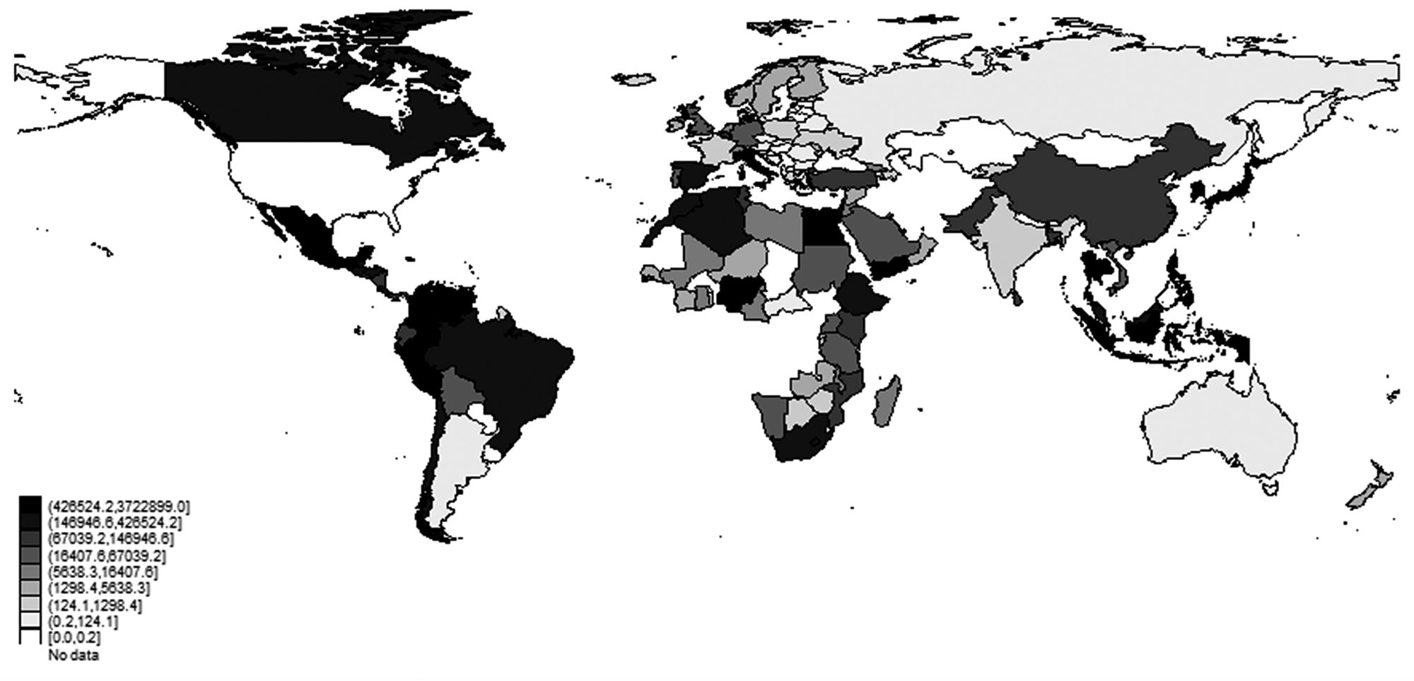
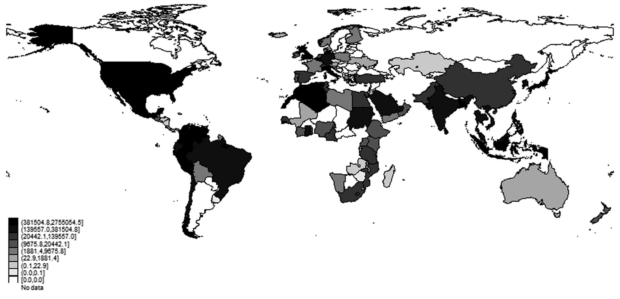
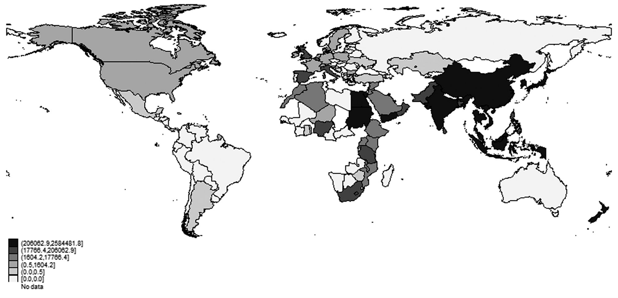
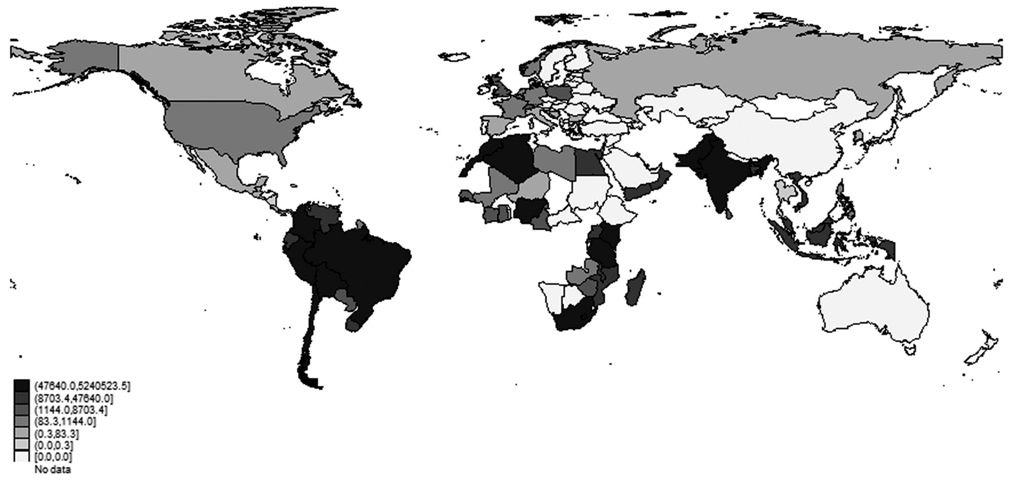
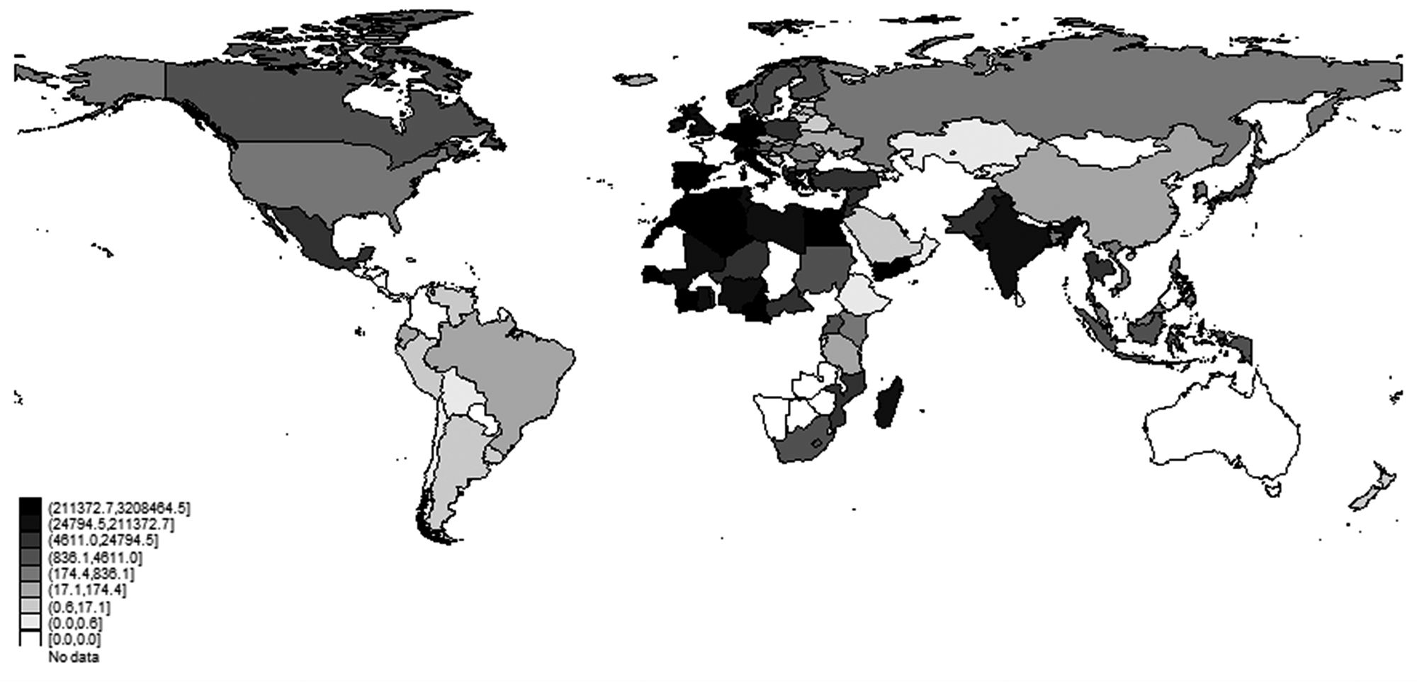
The situation in 2010 was one of more importers and exporters than ever before. Therefore, not only has the wheat trade grown, it has also expanded dramatically in geographical terms. Of course, this is the consequence of a significantly more diverse geographical distribution of world wheat consumption –and, to a minor extent, of world wheat production. Several maps have been plotted in the appendix in order to show this phenomenon. Figures A.1, A.2, A.3 and A.4 illustrate the world distribution of wheat production and consumption in 2006-10. In addition, figures A.5 and A.6 show the geographical distribution of wheat exports in 2006-10 (total and per capita respectively), and figures A.7 and A.8 do the same with imports¹. As can be observed, wheat is extensively consumed all over the world, this fact being true even in regions where its production is virtually negligible –most notably in the countries closest to the equator. These figures also suggest that certain variables, such as the country size, should necessarily be taken into account when trying to explain the world wheat trade.

With regard to the bilateral trade flows, figures 5 to 9 have been plotted to illustrate the main recipient countries of the exports proceeding from the top-5 major exporters in 2006-10: the United States, Canada, Australia, Argentina, and France. As expected, these maps clearly show the importance of distance and proximity. While Argentina’s exports are mostly directed to South American countries, Australia exports most of its wheat to Asia. Wheat produced in France is typically acquired by other European countries and by many North African countries. Meanwhile, the United States and Canada export significant amounts of wheat to each other, but also to a great number of countries all over the world. Distance is, however, only one of the many variables that directly affect trade. Section 4 is aimed at identifying and quantifying the impact that other major variables –such as income and production– have had on the international wheat trade.

3. International Trade Theories and the Gravity Equation

The GE emerged in the 1960s as a purely empirical proposition to explain aggregate gross bilateral trade flows (Fratianni, 2009). The seminal work of Timbergen (1962) paved the way for other empirical works, such as Pöyhönen (1963a, 1963b), Pulliainen (1963) and Linneman (1966). These works had few theoretical underpinnings, yet the relatively good fit of coefficient estimates suggested that some underlying economic law must be at work (Anderson, 2011). The basic idea behind the GE was that countries trade in proportion to their respective GDPs, and proximity. Therefore, the inspiration for the gravity model came from physics: countries trade in a similar way that planets are mutually attracted in proportion to their size and closeness, according to the Newtonian theory of gravitation. The most basic GE for bilateral trade flows is frequently specified as follows:

X_ij = Y_iY_j / d²_ij

A mass of goods supplied at origin i, Y_i, is attracted to a mass of demand for goods at destination j, Y_j, but the potential flow is reduced by the distance between i and j, d_ij. The predicted movement of goods between both countries would be X_ij. It is noteworthy that the most prominent models of international trade in the 1960s paid little attention to the distance and to the size of the economies involved in trade (WTO, 2012). While the Ricardian model focused on differences in technology across countries to explain trade patterns, the Heckscher-Ohlin (HO) model emphasized the role of factor endowments (WTO, 2012). There was little room for distance and size in traditional explanations of trade, and it is for this reason that the GE was thought of as a mere representation of an empirically stable relationship, and was considered to be an intellectual orphan, unconnected to the rich family of economic theory (Anderson, 2011: 1).

Yet this would change in the late 1970s, when the gravity model was legitimized by a number of theoretical works demonstrating that the basic GE could be derived from a range of standard trade theories (Deardorff, 1998). The first important attempt to provide theoretical micro-foundations for the gravity model was Anderson (1979). His contribution was based on a model of complete specialization and identical consumer preferences, and it was criticized at the time because the cornerstone of the theory seemed to have been constructed ad hoc (Deardoff, 1984: 503; Baldwin & Taglioni, 2006: 1). Anderson’s work was the first of many contributions that aimed to provide a theoretical basis for the GE. For instance, Baldwing and Taglioni pointed out that the emergence of the “new trade theory” in the late 1970s and early 1980s (e.g. Krugman 1979, 1980, 1981; Helpman, 1981) started a trend where the gravity model went from having too few theoretical foundations to having too many (Baldwing & Taglioni, 2006: 2). In fact, as Fratianni (2009) has noted, the GE has been derived from models of complete specialization (Bergstrand, 1985, Deardorff, 1998) but also from models of product differentiation with monopolistic competition (Helpman, 1987), models of incomplete specialization and trading costs (Haveman & Hummels, 2004) and hybrid models of product differentiation and different factor proportions (Bergstrand, 1989; Evenett & Keller, 2002).

The GE has become the “workhorse” of the applied international trade literature (Baldwing & Taglioni, 2006; Shepherd, 2012). Yet it is somewhat surprising that, despite its robust findings and empirical success, most economists and international trade theorists tended to ignore it until very recently. For instance, according to Anderson (2011), gravity first appeared in textbooks in 2004 (Feenstra, 2004). In 1995, Levinsohn and Leamer asserted that textbooks continue to be written and courses designed without any explicit references to distance, but with the very strange implicit assumption that countries are both infinitely far apart and infinitely close, the former referring to factors and the latter to commodities (Levinsohn & Leamer, 1995; Anderson, 2011: 1). Fortunately, recent research on the theoretical basis of GE has highlighted the importance of deriving the specifications and variables used in the gravity model from economic theory in order to draw the proper inferences from estimations using the gravity equation (WTO, 2012: 105). Hopefully, all those contributions will encourage the ongoing but difficult task of integrating empirics with theory. Our empirical case is, of course, very specific, since it is aimed at explaining trade in a particular commodity rather than analyzing aggregated trade flows.

We will make use of the GE in its simplest form in order to explain wheat trade flows between pairs of countries, in terms of the countries’ incomes, distance, and a host of idiosyncratic factors such as common language and common border. Several models will be estimated in order to include a number of control variables such as wheat production (both absolute and per capita) of both the importing and the exporting country. We will also be sensitive to the most recent critiques and recommendations in the GE literature, in order to make the most adequate estimation possible. First, Anderson and Wincoop (2003) show that controlling for relative trade costs is key for a well-specified gravity model. The main problem is that the so-called multilateral trade resistance terms (MTRs) are not directly observable. Many alternatives have been proposed to deal with this problem since the publication of Anderson and Wincoop’s work, one of them being the inclusion of a proxy variable for “remoteness”. In our case, we have chosen the simplest –yet widely-used– solution: the inclusion of country fixed effects for importers and exporters. All estimated models include a set of dummy variables equal to unity each time a particular importer appears in the dataset. Following this approach, we aim to account for all sources of unobserved heterogeneity that are constant for a given importer across all exporters. By also including a set of dummy variables equal to unity each time a specific exporter appears in the dataset, we account for all sources of unobserved heterogeneity that are constant for a given exporter across all importers. As far as the estimation procedure is concerned, Santos Silva and Tenreyro (2006) provide solid arguments for preferring the Poisson quasi-maximum likelihood estimator (PPML) over the ordinary least squares estimation (OLS) and the log-linearization approach when estimating a gravity equation. We will use the PPML because, following these authors, it has at least three noticeable advantages over other methods. First, it is consistent with the presence of fixed effects. Second, this estimator allows for the inclusion of observations for which the observed dependent variable (in this case, wheat imports) is zero. And third, the coefficients of any independent variables entered in logarithms can be interpreted as elasticities (WTO, 2012). An additional reason for preferring PPML over other estimation methods is that it produces estimates in which, summing across all partners, actual and estimated total trade flows are identical (Arvis & Shepherd, 2011: 1). According to these authors, Poisson is the only quasi-maximum likelihood estimator that preserves total trade flows, thus solving the “adding up” problem faced by other gravity model estimators.

In addition, our estimation method produces standard errors that are robust to arbitrary patterns of heteroskedasticity in the data. Since errors are likely to be correlated by country pair, we allow for clustering by country pair by specifying a clustering variable that separately identifies each pair of countries, regardless of the direction of trade: distance. Here, we use the method of Santos Silva and Tenreyro (2010) to identify and drop regressors that may cause the non-existence of the (pseudo) maximum likelihood estimates.

4. Data description and estimation

Our dataset has been constructed to account for the maximum percentage of total wheat trade while minimizing the number of zero values. Since many countries do not export any wheat, they have been dropped –as exporters– from the database. A large number of small countries whose imports are consistently null have also been dropped. Data on wheat imports for other countries is sometimes available only from a certain year onwards, so years with no data have been excluded. The final result is a non-balanced panel with 111 importers, 61 exporters, and 199,980 observations. From those observations, 167,689 have non-missing values in every explanatory variable that has been incorporated into the econometric models: gross domestic product of the importing and the exporting countries (both absolute and per capita), wheat production of the importer and the exporter (both absolute and per capita), distance, common language, contiguity, regional trade agreements in force, and World Trade Organization membership. The dataset accounts for an average of 70.31% of the total wheat trade between 1963 and 2010, and includes the most populous countries from every continent (see tables 1 and 2, in the appendix²). As Figure 10 illustrates, the coverage is slightly better from the 1990s onwards.

FIGURE 10

Total wheat trade (tonnes, area graphs, first axis) and total bilateral flows included (%, second axis), 1963-2010

Note: wheat also includes wheat flour.

Source: author’s elaboration from FAO (2016) and United Nations (2016).

The results from the estimation of seven different models are shown in Figure 11. The following dummy variables are included in every model: contiguity, common language, trade agreement in force, bothwtopre1994 and bothwtopost1994. Distance and the importing country GDP is also included in every regression. However, the seven different models find their reason to be on the decision to omit or include the remaining explanatory variables: GDPexporter, GDPpcimporter, GDPpcexporter, ProductionIMP, ProductionEXP, ProductionpcIMP, and ProductionpcEXP. Since some of the latter variables are indeed closely interrelated, the comparison of the seven models allow us to settle our conclusions on safer grounds. The seven proposed models fit the data relatively well: the R2 is always above 0.5, which means that the explanatory variables account for over half of the observed variation in trade.

This dataset was originally developed by Keith Head, Thierry Mayer, and John Ries (2010). As usual, contiguity is a dummy variable that takes the value 1 if the importer and the exporter share a common border and zero otherwise. Common language is a dummy variable equal to 1 if both countries share a common language. Bilateral distance has also been taken from Geodist, the CEPII distance dataset (Head, Mayer & Ries, 2010; Head & Mayer, 2014). Information on the existence of bilateral relationships (trade agreement in force) has been taken from Sousa (2012). This is a dummy variable that takes the value 1 if there was a bilateral trade agreement in force between the importing and the exporting country in a selected year, and zero otherwise. World Trade Organization (WTO) membership of different countries over time comes from the CEPII gravity set, which in turn is based on the information provided on the WTO official website. Since trade in wheat came to be under the WTO treatment only after the Uruguay round of negotiations, two dummy variables have been included; bothwtopre takes the value 1 if both the importing and the exporting country were WTO members before 1994 and zero otherwise; bothwtopost takes the value 1 if both the importing and the exporting country were WTO members between 1995 and 2010, and zero otherwise. Data on GDPs is expressed in real terms (1990 Int. Geary–Khamis $) and has been obtained from the Maddison-Project database (see Bolt & Zanden [2014] for more information on the underlying methodology). For certain years and countries, this information has been complemented with data on GDP growth from the World Development Indicators database (2016). Data on population also comes from World Bank (2016). Finally, data on wheat production is measured in real terms (tonnes) and comes from FAO (2016).

The first model is the most basic gravity equation possible. The main problem is that the coefficients of the two masses (i.e. GDPimporter and GDPexporter) are hardly interpretable because several relevant variables have been omitted –and these variables are strongly correlated to absolute GDPs. This is fixed in the second model, which also includes the GDP per capita of both the importer and the exporter. The positive and statistically significant coefficient in GDPimporter is now suggesting that the size of the destination market acts as an attraction force for wheat imports. As countries grow, they tend to import more wheat. Despite that this result was expected, it confirms our belief that absolute economic growth in importing countries –which is, of course, strongly related to their population growth– is key to understanding the great progress in total wheat trade that occurred between 1963 and 2010. However, this observation should be nuanced by taking into account the strong, negative, and statistically-significant coefficient in GDPpcimporter. While larger (more populous) countries tend to import greater amounts of wheat, rising per capita income may actually reduce imports via lower wheat demand per capita. This result is consistent with studies showing that the income-elasticity of demand for wheat not only tends to be highly inelastic, but that it is usually negative above certain levels of income (Fabiosa, 2011; FAPRI, 2009; Seale, Regmi & Bernstein, 2003). With regard to the exporter GDP, the unexpected negative sign probably has much to do with the fact that applying the logic of the gravity equation to the study of trade in individual commodities is not entirely straightforward. More specifically, absolute GDPs are not necessarily good proxies for supply. That is the reason why models 3 to 7 have been estimated: all of them include some other indicator of supply for the exporting country, either absolute wheat production or per capita wheat production. When supply is measured by absolute wheat production in the exporting country –rather than by its absolute GDP– the estimated coefficient is always positive (above 0.7) and statistically significant. The same is true if supply is proxied by per capita wheat production (in this case, the coefficients are even higher than 0.7). These results confirm the idea that, as countries produce more, they tend to export more wheat –the size of the market matters– and the idea that countries that become more specialized/more efficient in wheat production also tend to export more. It is important to note that countries with higher per capita wheat production are more likely to have enough wheat to satisfy domestic demand, thus making wheat surpluses available for export.

Models 3 to 7 also include some indicator of production in the importing country (absolute wheat production or per capita production). These variables are incorporated to control for the so-called home bias effect (Anderson & Wincoop, 2003). As Dal Bianco et al. (2016) do for the case of wine, we consider home bias in the context of wheat trade as the resistance to importing foreign products due to the supply of national products. Since the estimated coefficients for wheat supply in the importing country are negative and statistically significant, we may conclude that a home bias effect has existed in the world wheat trade. Finally, some other facts deserve special attention. As mentioned before, the exporter GDP is not a good proxy for wheat supply. Yet, when controlling for GDPpcexporter (as in models 2 and 7), the estimated coefficient in the exporter GDP remains negative and statistically significant, and is therefore telling us something: the size of the export market affects wheat exports negatively. This result is consistent with the hypothesis that, as countries grow, they tend to hold back production. If absolute GDP growth is partially due to population growth, a larger domestic market indeed means a higher domestic demand for wheat (thus leaving less of a wheat surplus for export). When it comes to the per capita GDP of the exporter, the findings are quite clear: as countries become richer, they tend to export larger amounts of wheat. This could be due to several facts. First, as countries grow, they usually enjoy higher land and labor productivity rates in agriculture. However, the positive and statistically-significant coefficient in the GDP per capita of the exporter remains high, even when controlling for its per capita wheat production (see model 7). This means that the greater wheat exports associated with income growth may have something to do with the demand side: as countries become richer, their population begins to substitute wheat for the consumption of other products, thus leaving growing wheat surpluses for export. Another possible interpretation is related to policies and international trade negotiations. As mentioned in the first section of this paper, wheat policies in exporting countries have usually involved trade-distortive instruments, such as export subsidies. It is well-documented that the United States (the country with the highest GDP per capita after Second World War according the Maddison Project [2013]) was able to mold GATT rules to its advantage in order to allow its interventionist wheat programs (Hathaway, 1987; Johnson, 1991). On these grounds, it seems reasonable to argue that income growth may lead to greater bargaining power in international trade negotiations, resulting in a greater ability to impose export subsidies and dump wheat surpluses abroad.

With regard to distance and the other control variables, first it must be said that their coefficient estimates seem to be less sensitive to the omission and incorporation of other important variables. A first conclusion may be drawn from the observed estimation results: distance and proximity really matter. For geographical contiguity, we find that countries that share a common border trade significantly more than those that do not³. In addition, the coefficient on distance is negative and statistically significant in every single model. The seven different estimations reveal that a 1% increase in distance tends to reduce wheat trade by roughly 1%. When it comes to cultural proximity –measured by the existence of a common language– we also find it to be a significant trade enhancer. Finally, with regard to the international trade organization, we find that the inclusion of wheat trade under the WTO umbrella –following the Uruguay round of negotiations– did not significantly alter the functioning of world wheat markets. On the contrary, it seems that the wheat trade has traditionally been fostered only by bilateral trade negotiations and agreements.

5. Conclusions

The history of the wheat trade over the second half of the twentieth century should not be considered as merely a history of successive international exchanges in a single commodity. Behind the observed trends in wheat trade flows, there are indeed countless national and international developments that constitute in themselves the very political and economic history of humanity, with all its complexity. There is no doubt that events such as the fall of the Berlin Wall, and international dynamics such as Cold War politics, have deeply affected international wheat trade. In fact, the market for wheat has often been crucial for national economic policy and development strategies, and it has been so for notable reasons. First, wheat-based products are a staple in many parts of the world, thus making the functioning of wheat markets a key element as far as national food security strategies are concerned. In some cases, if the expenditure share in wheat products was sufficiently high, wheat prices could be considered as a key element in determining real wages. For instance, after Second World War, this notion underlay certain development strategies based on promoting cheap wheat imports, with the aim of fostering industrialization. Second, wheat is not only extensively consumed, but also widely cultivated all around the world. This means that wheat prices not only significantly affect the economic welfare of consumers, but also, and sometimes very intensely, the revenues of a great number of primary producers. Since both consumers and producers vote –not to mention the usual ability of wheat growers to exert political pressure by other means– wheat policies have often been an extremely delicate matter of dispute, both within and between countries. Wheat policies –and especially commercial policies– in importing and exporting countries have commonly been designed to pursue a range of different goals, varying from assuring farm incomes to solving balance of payments problems, or achieving food security (or self-sufficiency). The observed trends in the volume and direction of wheat trade flows have surely been affected by those national historical contexts and policies, which were sometimes rooted in the interwar period –or even before. All these considerations have been thoroughly analyzed in González Esteban (2018), but are extremely difficult to quantify, let alone to incorporate into an econometric model. The major aim of this paper has been to show that a great percentage of the observed variation in wheat trade between 1963 and 2010 may actually be explained by certain standard economic variables, such as distance and GDP growth.

First, our estimation provides a confirmation for Anderson and Wincoop’s concept that the death of distance is exaggerated (Anderson & Wincoop, 2004: 1). In the case of wheat, it is clear that countries tend to trade more if they are closer to each other. The same is true if the importing and the exporting countries share a common border and a common language. Therefore, in a world characterized by an apparently growing integration between economies, both geographical and cultural proximity have still been important in explaining the direction of wheat trade flows. This can be seen most clearly in figures 5 to 9, which illustrate how the top 5 exporters (the United States, Canada, Australia, Argentina, and France) sell much more wheat to countries that are closer to them.

Second, our analysis shows that international wheat exchanges have depended much more on bilateral arrangements between countries than on the new multilateral organization of trade. The existence of good bilateral relationships between the importer and the exporter –measured by the existence of any kind of trade agreement between them– have shown positive results in terms of the total amount of traded wheat. However, it seems that the Uruguay round of negotiations and the incorporation of the wheat trade under the WTO organization did not significantly modify the actual organization of the world wheat trade.

Finally, with regard to the effect of income growth on the wheat trade, we have found it useful to control for relevant variables, such as income per capita and both absolute and relative wheat production. Doing so has allowed us to distinguish between different processes. With regard to the exporting countries, we find two different forces in operation. First, as countries grow, they tend to retain production in order to satisfy the growing domestic demand for wheat. However, if the process of economic growth is intensive rather than extensive (i.e. if we are talking about per capita GDP growth, rather than absolute GDP growth), then an export-enhancing force comes into play. This may be due to the lower per capita demand for wheat (wheat demand tends to be negative above certain levels of income), and/or to a greater ability to impose export-enhancing mechanisms such as export subsidies. With regard to the importing countries, we also find two different operating forces. Again, as countries grow, they require increasing quantities of wheat in order to satisfy domestic demand. Wheat imports can be reduced if population growth is accompanied by a growing domestic production (there is a home bias effect). And, if there is a process of intensive economic growth (i.e. per capita GDP growth) some import-limiting forces can also come into play, mostly the lower per capita wheat demand associated with dietary transitions and the substitution of wheat-based products for other sources of calories. However, caeteris paribus, population growth in importing countries act as a powerful import-enhancing force, and it surely is a crucial factor in explaining the tremendous growth in the wheat trade that occurred over the studied period.

Acknowledgements

I am deeply grateful to Professor Vicente Pinilla for his insightful comments and invaluable help in preparing this paper. I would also like to thank the anonymous reviewers of Historia Agraria. Lastly, financial support was provided by the Spanish Ministry of Economy and Competitiveness (project MEIC HAR2016-75010-R).

REFERENCES

Anderson, J. E. (1979). A Theoretical Foundation for the Gravity Equation. American Economic Review, 69 (1), 106-16.

Anderson, J. E. (2011). The Gravity Model. Annual Review of Economics, 3 (1), 133-60.

Anderson, J. E. & Wincoop, E. van (2003). Gravity with Gravitas: A Solution to the Border Puzzle. American Economic Review, 93 (1), 170-92.

Anderson, J. E. & Wincoop, E. van (2004). Trade Costs. Journal of Economic Literature, 42 (3), 691-751.

Anderson, K. & Nelgen, S. (2012). Updated National and Global Estimates of Distortions to Agricultural Incentives, 1955 to 2010.

Anderson, K. & Valenzuela, E. (2008). Estimates of Global Distortions to Agricultural Incentives, 1955 to 2007.

Anderson, K., Rausser, G. & Swinnen, J. (2013). Political Economy of Public Policies: Insights from Distortions to Agricultural and Food Markets. Journal of Economic Literature, 51 (2), 423-77.

Aparicio, G. & Pinilla, V. (2015). The Dynamics of International Trade in Cereals, 1900-1938. DT-SEHA, (1504).

Arvis, J. F. & Shepherd, B. (2011). The Poisson Quasi-Maximum Likelihood Estimator: A Solution to the “Adding Up” Problem in Gravity. MPRA Paper, (34334).

Baldwin, R. & Taglioni, D. (2006). Gravity for Dummies and Dummies for Gravity Equations. NBER Working Paper Series, (12516).

Bergstrand, J. H. (1985). The Gravity Equation in International Trade: Some Microeconomic Foundations and Empirical Evidence. The Review of Economics and Statistics, 67 (3), 474-81.

Bergstrand, J. H. (1989). The Generalized Gravity Equation, Monopolistic Competition, and the Factor-Proportions Theory in International Trade. The Review of Economic and Statistics, 71 (1), 143-53.

Bolt, J. & Zanden, J. L. van (2014). The Maddison Project: A Collaborative Research on Historical National Accounts. The Economic History Review, 67 (3), 627-51.

Callear, d. l. & Blandford, d. (1981). Food Security and the International Wheat Agreements. Cornell Agricultural Ecomomics Staff Papers, (81-11).

Dal Bianco, A., Boatto, V. L., Caracciolo, F. & Santeramo, F. G. (2016). Tariffs and Non-Tariff Frictions in the World Wine Trade. European Review of Agricultural Economics, 43 (1), 31-57.

De Hevesy, p. (1940). World Wheat Planning and Economic Planning in General. London: Oxford University Press.

Deardoff, A. (1984). Testing Trade Theories and Predicting Trade Flows. In R. W. Jones & P. B. Kenen (Eds.), Handbook of International Economics. 1: International Trade (pp. 467-517). New York: Elsevier.

Deardorff, A. (1998). Determinants of Bilateral Trade: Does Gravity Work in a Neoclassical World? In J. A. Frankel (Ed.), The Regionalization of the World Economy (pp. 7-32). Chicago: University of Chicago Press.

Eggleston, R. C. (1987). Determinants of the Levels and Distribution of PL 480 Food Aid: 1955-1979. World Development, 15 (6), 797-808.

Evenett, S. J. & Keller, W. (2002). On Theories Explaining the Success of the Gravity Equation. Journal of Political Economy, 110 (2), 281-316.

Fabiosa, J. (2011). Globalization and Trends in World Food Consumption. In J. L. Lusk, J. Roosen & J. F. Shogren (Eds.), The Oxford Handbook of the Economics of Food Consumption and Policy (pp. 591-611). Oxford: Oxford University Press.

Food and Agriculture Organization (FAO) (2016). FAOSTAT Statistics Database.

Food and Agricultural Policy Research Institute (FAPRI) (2009). FAPRI 2009 U.S. and World Agricultural Outlook. FAPRI Staff Reports, (09-FSR 1).

Feenstra, R. C. (2004). Advanced International Trade: Theory and Evidence. Princeton: Princeton University Press.

Fratianni, M. (2009). The Gravity Equation in International Trade. In A. M. Rugman (Ed.), The Oxford Handbook of International Business (pp. 72-89). 2nd ed. New York: Oxford University Press.

Friedmann, H. (1982). The Political Economy of Food: The Rise and Fall of the Postwar International Food Order. American Journal of Sociology, 88 (s1), 248-86.

Friedmann, H. (1990). The Origins of Third World Food Dependence. In H. Bernstein, M. McKintosh, Ch. Martin & B. Crow (Eds.), The Food Question: Profits versus People. London: Earthscan.

Ghoshray, A. (2006). Market Delineation and Price Leadership in the World Wheat Market: A Cointegration Analysis. Agricultural and Resource Economics Review, 35 (2), 311-26.

González Esteban, A. L. (2017). Why Wheat?: International Patterns of Wheat Demand, 1939-2010. Investigaciones de Historia Económica-Economic History Research, 13 (3), 135-50.

González Esteban, A. L. (2018). Patterns of World Wheat Trade, 1945-2010: The Long Hangover from the Second Food Regime. Journal of Agrarian Change, 18 (1), 87-111.

González Esteban, A. L., Pinilla, V. & Serrano, R. (2016). International Agricultural Markets after the War, 1945-60. In C. Martin, J. Pan-Montojo & P. W. Brassley (Eds.), Agriculture in Capitalist Europe, 1945-1960: From Food Shortages to Food Surpluses (pp. 64-84). London/New York: Routledge.

Hathaway, D. E. (1987). Agriculture and the GATT: Rewriting the Rules. Washington, DC: Institute for International Economics.

Haveman, J. & Hummels, D. (2004). Alternative Hypotheses and the Volume of Trade; The Gravity Equation and the Extent of Specialization. The Canadian Journal of Economics, 37 (1), 199-218.

Head, K. & Mayer, T. (2014). Gravity Equations: Toolkit, Cookbook, Workhorse. In G. Gopinath, E. Helpman & K. Rogoff (Eds.), Handbook of International Economics (pp. 131-95). Vol. 4. Amsterdam: Elsevier.

Head, K., Mayer, T. & Ries, J. (2010). The Erosion of Colonial Trade Linkages after Independence. Journal of International Economics, 81 (1), 1-14.

Helpman, E. (1981). International Trade in the Presence of Product Differentiation, Economies of Scale and Monopolistic Competition. Journal of International Economics, 11 (3), 305-40.

Helpman, E. (1987). Imperfect Competition and International Trade: Evidence from Fourteen Industrial Countries. Journal of the Japanese and International Economies, 1 (1), 62-81.

Institut International d’Agriculture (1947). Annuarie Internationale de Statistique Agricole 1941-42 á 1945-46. Volume II, Commerce International. Rome: Institut International d’Agriculture.

Johnson, D. G. (1991). World Agriculture in Disarray. London: MacMillan.

Krugman, P. R. (1979). Increasing Returns, Monopolistic Competition and International Trade. Journal of International Economics, 9 (4), 469-79.

Krugman, P. R. (1980). Scale Economies, Product Differentiation and the Pattern of Trade. The American Economic Review, 70 (5), 950-59.

Krugman, P. R. (1981). Intraindustry Specialization and the Gains from Trade. Journal of Political Economy, 89 (5), 959-73.

Levinsohn, J. & Leamer, E. E. (1995). International Trade Theory: The Evidence. In G. M. Grossman & K. Rogoff (Eds.), Handbook of International Economics (pp. 1339-94). Vol. 3. Amsterdam: Elsevier.

Linneman, H. (1966). An Econometric Study of International Trade Flows. Amsterdam: North-Holland.

Malembaum, W. (1953). The World Wheat Economy, 1885-1939. Cambridge: Cambridge University Press.

McCalla, A. F. (1966). A Duopoly Model of World Wheat Pricing. American Journal of Agricultural Economics, 48 (3), 711-27.

Morgan, D. (1979). Merchants of Grain. New York: The Viking Press.

Perkins, J. H. (1997). Geopolitics and the Green Revolution: Wheat, Genes and the Cold War. New York: Oxford University Press.

Pöyhönen, P. (1963a). A Tentative Model for the Volume of Trade between Countries. Welwirtschaftliches Archiv, 90 (1), 93-100.

Pöyhönen, P. (1963b). Toward a General Theory of International Trade. Economiska Samfundets Tidskrift, (16), 69-77.

Pulliainen, K. (1963). A World Trade Study: An Econometric Model of the Pattern of the Commodity Flows of International Trade in 1948-60. Economiska Samfundets Tidskrift, (16), 78-91.

Santos Silva, J. M. C. & Tenreyro, S. (2006). The Log of Gravity. Review of Economics and Statistics, 88 (4), 641-58.

Santos Silva, J. M. C. & Tenreyro, S. (2010). On the Existence of the Maximum Likelihood Estimates in Poisson Regression. Economic Letters, (107), 310-12.

Seale, J. L., Regmi, A. & Bernstein, J. A. (2003), International Evidence on Food Consumption Patterns. United States Department of Agriculture Technical Bulletin, (1904).

Shepherd, B. (2012). The Gravity Model of International Trade: A User Guide. Bangkok: ARTNeT, United Nations.

Sousa, J. de (2012). The Currency Union Effect on Trade is decreasing over Time. Economic Letters, 117 (3), 917-20.

Son, J. S. (1986). Wheat Imports and Cheap Food Policy in Korea. Master’s thesis. East Lansing: Michigan State University.

Maddison Project (2013). Maddison Project Database Version 2013.

Tinbergen, J. (1962). Shaping the World Economy: Suggestions for an International Economic Policy. New York: Twentieth Century Fund.

United Nations (2016). UN Comtrade Database.

Winders, B. (2009). The Politics of Food Supply: U.S. Agricultural Policy in the World Economy. New Haven: Yale University Press.

World Bank (2016). World Development Indicators.

World Trade Organization (WTO) (2012). A Practical Guide to Trade Policy Analysis. Genève: United Nations Conference on Trade and Development/World Trade Organization.

↩︎ 1. See Appendix, DOI:

↩︎ 2. See note 1.

↩︎ 3. The coefficients estimated for the discrete variables may be interpreted as semi-elasticities: 100*[exp( β i)-1].